


The ISO 26262 automotive safety standard requires evaluation of safety goal violations due to random hardware faults to determine diagnostic coverages (DC) for calculating safety metrics. Injecting faults using simulation may be time-consuming, tedious, and may not activate the design in a way to propagate the faults for testing. With formal verification, however, faults are easily categorized by structural analysis providing a worst-case DC. Furthermore, faults are analyzed to verify propagation, safety goal violations, and fault detection, providing accurate and high confidence results. This article describes in detail how to run a better fault campaign using formal.
ISO-METRICS
The automotive functional safety standard, ISO 26262, defines two verification requirements for integrated circuits used in automotive applications—systematic failure verification and random hardware failure verification. Systematic failures are design bugs found with typical functional verification. Random hardware failure verification is where faults are injected into a design to test assumptions about the design’s safety mechanisms to see if they work. Just as functional verification uses coverage to determine completeness, the ISO standard defines a form of coverage for random hardware failures called diagnostic coverage, which represents the percentage of the safety element that is covered by the safety mechanism.
Diagnostic coverage is computed by first determining the number of different types of faults in a design. If a fault is injected and has no impact on the safety critical goal (function) or output, then it is considered safe. Likewise, any fault injected that can be detected or notified to the car driver is also considered safe. What we are really looking for are those faults that are either unprotected by any safety mechanism (known as a single-point fault) or are supposed to be covered but a safety mechanism that fails to detect it (referred to as a residual fault). The ISO standard also addresses potential faults in the safety mechanism. Typically, an automotive design will have a secondary safety mechanism like POST to check the behavior of the primary safety mechanism. In order to test the safety mechanism is correct, a fault must be injected into the design to activate the primary safety mechanism, and then a second fault injected into the primary safety mechanism to see if it still works. This is referred to as a dual-point fault, which falls into the multi-point fault category (though the standard only requires testing at max 2 faults unless there is an architectural reason to test more). Any dual-point fault not covered by the secondary safety mechanism is considered latent.

Once all the faults in a design are classified, then the ISO 26262 metrics are easy to compute. Often, fault counts are rolled up together in an FMEDA[1] to compute the single-point fault metric (SPFM) or latent fault metric (LFM). Alternatively, the diagnostic coverage can be computed as a percentage and then used in the FMEDA in combination with process FIT[2] rates (λFIT) for specific failure modes[3]. (See [1], sections C.1-C.3 for details on the ISO metric calculations).
WHAT’S IN A NAME?
Electronics in cars have always been treated as black boxes—when a part fails, the part is swapped with another. So when the ISO standard refers to a safety element and a safety mechanism, they traditionally have been treated as discrete components, making safety components rather obvious.
Technology, however, allows us to squeeze everything into an IC, blurring the lines between a safety and non-safety related component. For example, registers may be shared between different safety and non-safety related parts of the design. This complicates matters because only safety related elements should be used in calculating fault metrics, but by mixing safety/non-safety logic together, the entire design becomes a safety component. The only way to justify removing non-safety related logic is to show there is independence between the safety and non-safety logic, which can be done using a dependent failure analysis (DFA). Proving independence, however, is typically not easy, and including all design logic means injecting more faults than necessary, which will most likely dilute the diagnostic coverage.
Instead of identifying safety elements in an IC (since logic probably spans multiple modules), it is easier to identify safety critical paths that when combined together form the safety goal or safety function. Likewise, a fault may be detected by multiple safety mechanisms, any of which may amount to the fault being detected or perceived. Therefore, on an IC, the idea of a safety element has less to do with module boundaries and more to do with related safety logic, perhaps more accurately referred to as a safety domain.[4]
THE CAMPAIGN TRAIL
Assuming all safety mechanisms have been fully functionally verified, then it is time to perform random hardware testing or what is known as a fault campaign. Depending on the high-level safety concepts, multiple fault campaigns may need to be performed, one for each type of failure mode (usually stuck-at0, stuck-at1, or transient failure modes).
There are four steps necessary for a fault campaign. First, faults need to be activated. In an RTL design, all nets, registers, and ports are possible faults. While this is a lot of faults, there are many times more in a gate-level netlist (in the millions). The number of possible faults becomes astronomical when considering dual-point faults for latent fault analysis. Practically, simulations take too long to possibly test all faults. Instead, a random sampling of potential faults are chosen (usually several thousand), and simulated in order to give a statistically acceptable margin of error in the campaign results.
The second step is to propagate the fault through the design. While regression tests can be used for fault injection, extra effort should be made to ensure that the faults actually propagate. For example, if the design logic is in the wrong state, then propagation of the fault may not be possible. This either requires a bit of manual effort and inspection, use of coverage metrics, or turning a blind eye to the fact that the tests selected may have been totally useless. In other words, simulation results may provide high confidence from a statistical sampling perspective, but they don’t provide high confidence that the results are actually meaningful.
The third step is to observe the fault, or indicate that the fault has been controlled or detected. Testbenches are great at checking and indicating failures; however, this can become a hindrance in a fault campaign. Injecting random faults means that the simulation may go off into the weeds and failure out before the fault can even propagate to be detected. Often, tests are compared with a golden simulation waveform (i.e., one without the fault injected), and the test is considered a failure if the safety outputs differ. Unfortunately, the assumption here is that a different output implies a fault. It is also possible that injecting a fault causes the design to go down another path that is legal. Likewise, the safety functions and mechanisms may differ in the waveform, but the safety mechanism may actually detect the failure. The test may be marked as failing when in fact it should be considered successful. Conversely, a test may end with a passing result because no checker fired, but the fault went undetected so the test should be counted as a failure. Therefore, results need to be interpreted, as well as the fault detection interval(FDI) considered, which specifies a maximum amount of time for a fault to propagate to detection before it is considered unsafe.
Lastly, the fourth step is to report the results. In an IC where resources are shared, the results of the fault injection need to be merged. For example, suppose a safety function is composed of multiple safety critical paths through the design as shown in Figure 1. The fault has no impact on path 1, which would imply the fault is safe. However, down path 2, the fault goes undetected by the safety mechanism, i.e., it is a residual fault. In this example, the residual fault of path 2 would have priority over the safe results of path 1 so the merged result would be considered as a residual fault. The priority of the faults can be inferred from the flow chart B.2 in the part 5 of the ISO standard[2].
Figure 1 – Merging Fault Campaign Results:
 |

WORK SMARTER, NOT HARDER
Working smarter is where formal comes in. Formal has to synthesize a design into a Boolean representation in order to perform its analysis. The size of the design does not matter, but only that the design is synthesizable. This allows the formal tool to be able to trace back the cone of influence of a signal, i.e., all the logic that can possibly affect it. In the context of a random hardware failure analysis, a cone of influence (COI) can automatically prune out all faults that are structurally safe without requiring further analysis since anything outside of the cone is by definition classified as a safe fault, shown in Figure 2, below. Further, the cones of influence can reveal what logic is covered by a safety mechanism or not, indicating single-point, residual, and latent faults. This structural analysis provides a quick classification before any fault injection is performed, which provides a worst-case or best-case scenario for the diagnostic coverage calculation.
Figure 2 – Formal Cones of Influence (COI):
") |
Further structural fault pruning can be done by looking at the minimum number of cycles that faults require to propagate through the design. If the propagation time is greater than the fault detection interval or multi-point fault detection interval specified by hardware requirements, then it is by definition undetectable and classifiable without further analysis. Additional faults can be pruned by constraining the design, which will cause the formal synthesis to prune logic just like a synthesis tool. Lastly, given the appropriate formal engine, faults could be collapsed if they can be proven to be structurally equivalent or dominant, much like an ATPG algorithm.
Structural analysis is typically pretty quick, and results in a worst-case/best-case diagnostic coverage calculation are shown in Figure 3, below. In this example, 286 state bits reside outside of the cone of influence in this RTL module so they are automatically classified as safe. Other state bits are classified as residual or dual-point faults, but without further analysis, it is not verified. They are marked as unverified because structurally they may look like a particular type of fault, but there is no guarantee once the fault is injected that it will affect the safety goal or be detected. To move these faults into the verified category, formal analysis needs performed. Assuming the worst case scenario that all the dual-point faults in the safety function are residual, a worst-case residual diagnostic coverage can be calculated. Likewise, assuming all dual-point faults in the safety mechanism are latent, a worst-case latent diagnostic coverage can be computed. That means if your safety ASIL goal is only ASIL-B (90%), then no further analysis is required for residual faults since structurally the coverage cannot be worse than 91%. On the other hand, a latent diagnostic coverage of 20% is below an ASIL-B level (60%) so latent fault analysis is necessary.
Figure 3 – Results from Structural Analysis:
 |
BESIDES MYSELF
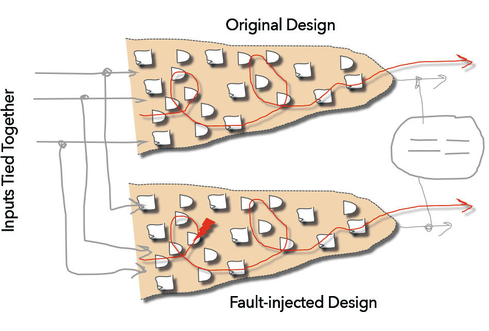
Using formal’s structural analysis greatly helps with the first major challenge in a fault campaign—reducing the number of faults that need to be activated. The second major challenge is propagating the fault through the design. As mentioned before, proving that a fault really propagates through a design in simulation is not a trivial matter. With formal, however, fault propagation is guaranteed. Formal exhaustively traverses through the state space, finding whatever path possible to prove or disprove whether a fault can propagate. No manual inspection, hand-crafting of tests, or writing of covergroups is required to guarantee that the fault sensitized the path to the safety function or safety mechanism. Better yet, formal does not require stimulus to be given to it, nor is a testbench required. The formal tool automatically determines the stimulus. In traditional formal verification, formal exhaustively goes down all paths, including illegal or undefined states, which results in false negatives. For fault propagation, however, a specialized formal app called Sequence Logic Equivalency Checking (SLEC) can be used.
SLEC can be used to prove two designs are equivalent, but unlike LEC (logic equivalency checking), which checks only that the combinational logic between registers is equivalent, SLEC checks that the functional outputs of two designs are equivalent. In other words, the designs can be implemented totally differently with different internal timing as long as their outputs are the equivalent. SLEC automatically ties the inputs together, applies the stimulus, and then checks that the outputs are the same. SLEC has many uses like checking that a design was ported from VHDL to Verilog correctly, or that adding extra logic to a design does not affect the main functionality (like the use of chicken bits).
In a fault campaign, SLEC provides the mechanism to constrain the inputs without any user input. The design under test is compared with itself, and a fault is injected into its other instance. If the fault does not cause the outputs to change (i.e., the two instances are equivalent even when the fault is injected), then the fault cannot violate the safety goal and is proven safe. Since the inputs are tied together, the formal inputs are constrained by the original design; i.e., only legal values through the design can be sent through the error-injected instance. This eliminates any hand-crafted tests or constraints, and the state space can be exhaustively explored.
Figure 6 Key: (SF = safe fault, SPF = single-point fault, RF = residual fault, and DPF = dual-point fault).
Figure 4 – Fault Propagation Using Sequence Logic Equivalency Checking (SLEC):
") |
Injecting the fault with formal simply requires creating a conditional cutpoint. A cutpoint is a net or register whose driver has been removed that becomes a formal control point, which can be used to create a stuck-at or transient fault. SLEC also allows the use of cover properties so you can specify that when a specific fault is injected, a safety goal violation occurs and it is detected within a specified time interval.
Fault analysis using formal SLEC can be broken into three steps: (1) safe fault analysis, (2) residual fault analysis, and (3) latent fault analysis. Safe fault analysis is where a fault is injected and checked to see if it propagates through the design unconstrained. If the outputs remain equivalent, then the fault is proven safe. This is an easier proof for formal since residual fault analysis requires checking for a safety goal violation that is not detected within a specific time interval. Unconstrained SLEC is usually pretty fast, but most faults within a cone of influence are not likely to have no effect on a safety output. As shown in Figure 5, the safe fault increases since some of the dual-point faults in the safety function have been proven safe.
Figure 5 – Safe Fault Analysis Results:
 |
Next, residual fault analysis is performed using SLEC to see if all the dual-point faults in the safety function can be detected (Figure 6). Anything not detectable means that they are not covered by the safety mechanism and therefore a residual fault. Figure 7 shows how as the faults are verified, some may be proven to be residual or detectable, which narrows the range for the residual diagnostic coverage.
Figure 6 – Formal Flow for Safe and Residual Fault Analysis:
 |
Figure 7 – Residual Fault Analysis Results:
 |
DOUBLE TROUBLE
Figure 8 shows how as dual-point faults in the safety mechanism are verified as detectable, the latent diagnostic coverage range narrows to a more acceptable level.
Figure 8 – Latent Fault Analysis Results:
 |
Figure 9 – Latent Fault Analysis Flow:
 |
HOME ON THE RANGE
Of course, formal has its limitations. It requires a synthesizable design, which means some components maybe be black boxed. State-space and memory are the biggest limitations so typical formal techniques like breaking up the problem may need to be used. Likewise, it may be more practical to run on smaller blocks and roll up results into a larger FMEDA. For faults that do not converge in formal, they can be exported to simulation or emulation (formal can even generate simulation testbenches that target a particular activity) to be run with the normal regression.
The ability to immediately produce a diagnostic coverage range upfront in your fault campaign is one of the biggest advantages of using a formal-based flow. Formal also provides a better solution for the other fault campaign challenges.
It can significantly prune the number of faults required for analysis. The results are proven and exhaustive, which is not practical with any simulation or emulation flow. Faults are guaranteed to be activated, propagated, and observed. No labor intensive, hand-crafting of tests and testbenches is required, and the entire formal flow can be automated based off of nothing more than a few inputs describing the safety function signals and the safety mechanism. Lastly, adding dual-point faults or even random transient faults are simple with formal since it handles all the inputs. All reasons why formal is the better way to run a functional safety fault campaign.
REFERENCES
- [1] ISO 26262:5-2011. Road vehicles – Functional Safety — Part 5: Product development at the hardware level. International Standardization Organization.
- [2] ISO 26262:5-2018. Road vehicles – Functional Safety — Part 5: Product development at the hardware level. International Standardization Organization.
- [3] Doug Smith. How Formal Reduces Fault Analysis for ISO 26262. White Paper.
- [4] Avidan Efody. Picking Your Faults: Advanced Techniques for Optimizing ISO 26262 Fault Analysis. White Paper.